
Dynamics and computation
A dynamical system is a stateful system (often with a continuous state space) evolving over time. Thus, dynamical systems can be (and are being) used to capture the behavior of both natural and articifical systems over time. The state space of dynamical systems is typically continuous, which means that one has to look at continuous models of computation. Here is a short 2013 Communications of the ACM article I wrote explaining computation over the reals. There is also an older 2006 article with Stephen Cook in the Notices of the AMS.
There are at least two natural connections between dynamics and computation. In one direction, the question “which properties of which dynamical systems can be computed and how efficiently?” is foundational to mapping the limits of applied mathematics. In the opposite direction, “how powerful a computation can a given dynamical system simulate robustly?” touches upon the Church-Turing thesis and questions of hypercomputation.
- Which properties of dynamical systems can be computed? The case of Julia sets
- Dynamical systems as computational devices and the Space-Bounded Church-Turing Thesis
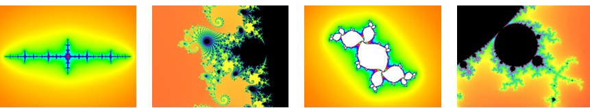
Julia sets are some of the most visualized objects in Mathematics. They arise in the study of complex dynamics (that is, the state space if the set $\mathbb{C}$ of complex numbers, visualized on the plane), along with the Mandelbrot set. From the scientific perspective, the family of Julia sets and the complex dynamics that gives rise to them, are sufficiently rich to exhibit phenomena one sees in the “wild”. At the same time, after 100+ years of deep study, we know a lot about them, making them good “lab models” for more general dynamical systems. Computer programs had been written to visualize Julia sets (by amateur programmers and professional mathematicians alike). Thus questions about computational properties of Julia sets are natural to consider, and may shed light on the broader set of phenomena we should expect in “computablility of dynamical systems”.
Consider the quadratic function $f_c:\mathbb{C}\rightarrow \mathbb{C}$ given by $f_c(z):=z^2+c$. For any initial point $z_0$, the mapping $f_c$ induces a (discrete-time) trajectory of the evolution of $z$ under $f_c$: $z_1=f_c(z_0)=z_0^2+c$, $z_2=f_c(z_1)=(z_0^2+c)^2+c$, and more generally $z_{t+1}=f_c(z_t)$.
This evolution, viewed as a dynamical system, raises quesitons of the form “what will happen to the trajectory eventually?” and “what can be said about the set of trajectories as a whole?”.
If $|z_0|$ is sufficiently large, e.g. $|z_0|>|c|+1$, then we will have $|z_1|>|z_0|$, and the trajectory will rapidly escape to $\infty$. On the other hand, if $z_0$ is a root of the polynomial $z^2+c=z$, then it will be a fixed point of the dynamical system, and its trajectory will not escape to $\infty$. The filled Julia set in this case is the set of initial conditions for which the dynamics does not escape to $\infty$: $$ K_c:=\lbrace z_0: z_t\nrightarrow\infty\rbrace. $$ The Julia set is the boundary of $K_c$: $J_c:=\partial K_c$. It is the set of points around which the long-term behavior is unstable: if $z\in J_c$, then any neighborhood of $z$ contains both points whose trajectories escape to $\infty$ and those whose trajectories stay bounded.

As it turns out, there exist non-computable quadratic Julia sets:
Theorem [BY'06]: There exists a parameter $c$ such that no Turing Machine with access to parameter $c$ can compute arbitrarily precise picture of $J_c$.
Moreover, it turns out that such a $c$ can be computed explicitly [BR07].
When a non-computability result is present, one might expect non-computability to be the rule, and computational tractability to be a lucky exception. Quadratic Julia sets are an interesting case-study, since they are rich enough to support many dynamically interesting behaviors, but are sufficiently well-understood to allow us to answer most questions about their computational properties. Surprisingly, non-computability sometimes occurs, but it is the exception.
In fact, by several measures, we either know that “most” quadratic Julia sets are computable, or strongly suspect that they are. Intuitively, the non-computable examples are constructed by carefully encoding a computationally difficult function into the parameter $c$ at infinitely many scales (more precisely, the encoding uses a continued fraction expansion). Perturbing $c$ by even a tiny amount will destroy most of this encoding.
Returning to the broader question of “which properties of dynamical systems can be computed?”, one can loosely calssify computational hardness results into two categories: “systems that can simulate generic computation” and “problems into which hard-to-compute functions can be carefully woven”.
If a dynamical system is rich enough to simulate a Turing Machine (and thus generic computation), then diagonalization results starting with the intractability of the Halting Problem and the time hierarchy theorems imply that the only way to answer questions about their long-term behavior is through simulation. Cellular automata generally belong to this category.
Even if a dynamical system is not rich enough to simulate generic computation, one can still carefully reduce some non-computable function to some long-term property of the dynamical system. It is very unlikely that all computation can be encoded into iterations of a fixed quadratic polynomial over $\mathbb{C}$), but we can carefully construct a $c$ such that computing arbitrarily high precision images of $J_c$ is as hard as solving the Halting Problem.
A closely related question is that of robustness. If we perturb the dynamical system a little bit, will the non-computability phenomenon disappear? One would expect the answer to be ‘yes’ in the second case, and ‘depends’ in the first case. If the non-computable example had to be carefully constructed, then noise is likely to destroy it (as it does in the case of quadratic Julia sets). More generally, what can be said about the computational complexity of noisy dynamical systems?
In full generality, this question is too philosophical to be precisely formulated as a purely mathematical conjecture. It is similar in flavor to the Church-Turing Thesis that asserts that all physically relevant dynamical systems are at most as powerful as a Turing Machine (or any other general-purpose computing device) for the purposes of computability. The best-known quantitative refinement of the CT Thesis, sometimes called the Extended Church-Turing Thesis (probably falsly – see quantum computing) extends the connection to time complexity: any computation by a dynamical system can be efficiently simulated in time polynomial in the size of the system and its original runtime. Relatively little attention has been given to space (that is memory) complexity in this context, even though memory complexity is a more robust notion, and is easier to interpret than time in the context of dynamical systems.
The reason that properties of dynamical systems under noise become computationally tractable is that in the presense of noise these systems are only able to maintain a limited amount of memory over time. A system capable of robustly representing only $2^M$ distinct states (corresponding to $M$ bits of memory) can be analyzed by a Turing Machine using only $poly(M)$ memory (though potentially in time exponential in $M$). How one might define the amount of “memory” a system has? Information theory comes in handy here.
Suppose the evolution of the system is given by the sequence $X_1,X_2,\ldots$, where $X_{t+1}$ is obtained from $X_t$ as $$X_{t+1}=N_\varepsilon(\Phi(X_t)),$$ where $\Phi(X_t)$ is the (noiseless) evolution rule, and $N_\varepsilon$ is a noise operator. We can define the memory of the system as: $$ M:= I(X_{t+1};X_t), $$ the amount of information the next step retains about the previous one.
The system’s dimension plays a critical role in the amount of memory it retains. If the state space of $X_t$ is bounded and has $d$ dimensions, then under random noise of magnitude $\varepsilon$ we should expect the memory to be $M\sim d\cdot \log (1/\varepsilon)$: memory scales liniarly in dimension but only logarithmically in the noise.
With a “definition” of memory at hand, we can postulated a space complexity version of the Church-Turing thesis. We call it the Space-Bounded Church-Turing thesis (SBCT):
Space-Bounded Church-Turing thesis [BRS'15]: A dynamical system with memory capacity $M$ is at most as powerful as a Turing Machine with $poly(M)$ bits of memory.
Unlike the extended-CT (which talks about time complexity), SBCT does not appear to contradict our current understanding of the limits of quantum computing. A stronger (and mathematically more formalizable) assertion is that whenever the noise itself is computationally simple (and thus is not a source of more computational complexity), long-term properties of a system with $M$ bits of memory can be computed by a Turing Machine with $poly(M)$ space. This indeed can be shown in some interesting special cases [BRS'17].
The SBCT is consistent with the fact that non-computability in the context of Julia sets is not robust to noise. The state space over which the dynamics defining the Julia sets operates is $\mathbb{C}$, with error $\varepsilon$ such a system only has $\sim\log (1/\varepsilon)$ memory. On the other hand, the memory of a cellular automaton (even with noise) scales with the size of its board (each cell can “remember” $\sim 1$ bit of information), which is typically infinite. Therefore, their long-term properties are potentially undecidable even in the presense of noise, again, consistently with SBCT.
Surveys on computing over the reals:
On Julia sets:
 Book: Computability of Julia Sets
Mark Braverman, Michael Yampolsky
Springer, 2009
[Amazon] [Springer]
On computability in dynamics more generally and the Space-Bounded Church-Turing thesis:
- A 2012 talk I gave at the 2012 Turing Centenary conference in Manchester.
- A phys.org article about the SBCT.